 |
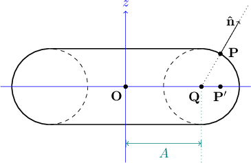
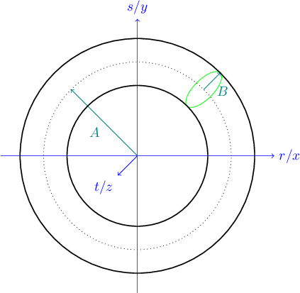
Figure 13.1: The torus dimensions $A$ and $B$. |
We now explore how to use the ray tracer code to draw a torus, which is more commonly known as a donut shape. This shape is implemented by class Torus, which is declared in imager.h and implemented in torus.cpp. Two constants suffice to define the shape of the torus: $A$, the distance from the center of the hole inside the torus and the center of its tube, and $B$, the radius of the tube, as shown in Figure 13.1. In order to ensure that there is a hole inside the torus, we will assume that $A > B$.
| |
|
Note that Torus is a reorientable solid (it derives from SolidObject_Reorientable), so it technically resides in object space coordinates $(r,s,t)$. However, I will use $(x, y, z)$ throughout the derivation here to more closely match the x, y, and z member variables of the C++ type Vector. Hopefully this will be more helpful than confusing when looking back and forth between the C++ code and the math in this chapter.
Our torus is centered at the origin $(0,0,0)$ and oriented such that it is cut in half (like a bagel) by the $xy$ plane. The following equation describes every point on the surface of a torus aligned this way. See the Wikipedia article Torus for more information about the derivation of this formula.
\[ (x^2 + y^2 + z^2 + A^2 - B^2)^2 = 4 A^2(x^2 + y^2) \]
As with every other kind of solid object we want to depict with the ray tracer code, we will need to solve equations for intersections with a ray, and figure out how to calculate a surface normal vector for an intersection point once we find it. This will be the most challenging of the algebra problems we have faced so far. As usual, we will substitute occurrences of $x$, $y$, and $z$ in the torus equation with linear expressions of the parameter $u$ based on the parametric ray equation $\mathbf{P} = \mathbf{D} + u \mathbf{E}$:
\[ \begin{cases} & x = E_x u + D_x \\ & y = E_y u + D_y \\ & z = E_z u + D_z \end{cases} \]
The substitution yields a single equation in $u$ that expresses where along the ray (if anywhere) that ray passes through the surface of the torus:
\begin{align*} & \left[ (E_x u + D_x)^2 + (E_y u + D_y)^2 + (E_z u + D_z)^2 + (A^2 - B^2) \right] ^2 \\ = \quad & 4 A^2 \left[ (E_x u + D_x)^2 + (E_y u + D_y)^2 \right] \end{align*}
Expanding the innermost squared terms that involve $u$, we find
\begin{align*} \big[ & (E_x^2 u^2 + 2 D_x E_x u + D_x^2) \\ + & (E_y^2 u^2 + 2 D_y E_y u + D_y^2) \\ + & (E_z^2 u^2 + 2 D_z E_z u + D_z^2) \big] ^2 \\ = \\ 4 A^2 \big[ & (E_x^2 u^2 + 2 D_x E_x u + D_x^2) \\ + & (E_y^2 u^2 + 2 D_y E_y u + D_y^2) \big] \end{align*}
Collecting like powers of $u$ on both sides of the equation, we have
\begin{align*} & \big[ (E_x^2 + E_y^2 + E_z^2)u^2 + 2(D_x E_x + D_y E_y + D_z E_z)u + (D_x^2 + D_y^2 + D_z^2 + A^2 - B^2) \big] ^2 \\ = \quad & 4 A^2 \big[ (E_x^2 + E_y^2)u^2 + 2(D_x E_x + D_y E_y)u + (D_x^2 + D_y^2) \big] \end{align*}
Let's define some constant symbols to simplify the algebra. Note that all of these definitions contain nothing but known constant terms, so the C++ algorithm will have no difficulty calculating their values.
\[ \text{Let } \begin{cases} \quad G&= 4 A^2 (E_x^2 + E_y^2) \\ \quad H&= 8 A^2 (D_x E_x + D_y E_y) \\ \quad I&= 4 A^2 (D_x^2 + D_y^2) \\ \quad J&= E_x^2 + E_y^2 + E_z^2 = \lvert \mathbf{E} \rvert ^ 2 \\ \quad K&= 2(D_x E_x + D_y E_y + D_z E_z) = 2(\mathbf{D} \cdot \mathbf{E}) \\ \quad L&= D_x^2 + D_y^2 + D_z^2 + A^2 - B^2 = \lvert \mathbf{D} \rvert ^2 + (A^2 - B^2) \end{cases} \]
The equation becomes much more concise:
\[ (J u^2 + K u + L)^2 = G u^2 + H u + I \]
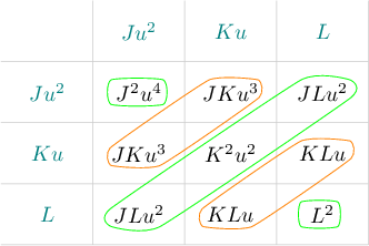
Expanding the squared term on the left is aided by a 3-by-3 grid showing every term multiplied by every term, as shown in Figure 13.2.
| |
|
Grouping the grid in upward sloping diagonals, as shown by the five curves in the figure, reveals collections of like powers of $u$. Summing the terms along these diagonals and factoring out the common powers of $u$, we have:
\begin{align*} & J^2 u^4 + 2 J K u^3 + (2 J L + K^2)u^2 + 2 K L u + L^2 = G u^2 + H u + I \end{align*}
Subtracting the right side of the equation from both sides and collecting like terms, the equation becomes:
\begin{align*} & J^2u^4 + 2JKu^3 + (2JL+K^2-G)u^2 + (2KL-H)u + (L^2-I) = 0 \end{align*}
An equation like this, where the unknown variable $u$ appears as $u^4$, $u^3$, $u^2$, $u^1$, and $u^0$ (the constant term $L^2-I^2$) is known as a quartic equation. It is solvable analytically, but the procedure is very complicated. I will not detail the solution here because there are many resources on the Internet that do a fine job. The source file algebra.cpp and its header file algebra.h contain a pair of overloaded functions called SolveQuarticEquation, one geared for quartic equations with all real coefficients (as we have here), and another more general version for those with complex coefficients. The complex version of SolveQuarticEquation is based on techniques from the Wikipedia article called Quartic equation. The real version calls the complex version and filters out any solutions that are not real numbers. Only real values of $u$ have meaning in the parametric ray equation, so we use the real version of SolveQuadraticEquation to solve the torus equation above.
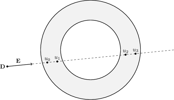
Take a look in torus.cpp at the method Torus::SolveIntersections. Given a vantage point and a direction vector, it finds all positive real solutions for $u$. Because the intersection equation is quartic in $u$, there can be up to four real solutions. This makes sense intuitively because a ray can pierce a torus in up to four places, marked $u_0$ through $u_3$ in Figure 13.3.
| |
|
Torus::SolveIntersections fills in the parameter uArray with 0 to 4 positive real solutions for $u$, and returns the number of solutions. The caller must use the return value to know how many of the elements of uArray are valid.
The Torus class derives from SolidObject_Reorientable so that the math can assume a fixed position and orientation in space, while still allowing us to create images of a torus translated and rotated any way we want. Torus::ObjectSpace_AppendAllIntersections receives a vantage point and direction vector that have already been translated into object space coordinates. It calls SolveIntersections to find 0 to 4 positive real values of $u$. Each valid value $u$ value gives us an intersection point when $u$ is plugged into the parametric ray equation $\mathbf{P} = \mathbf{D} + u \mathbf{E}$.
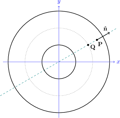
We are left with the problem of finding the surface normal unit vector for a point on the surface of a torus. It is possible to solve this problem using 3D calculus and partial derivatives, but with a little geometric intuition and a pair of diagrams, there is a much easier way. Figures 13.4 and 13.5 show two views of a point $\mathbf{P}$ on the surface of a torus, one edge-on, the other top-down.
| |
|
| |
|
In both views, $\mathbf{O}$ is the origin $(0,0,0)$, which is also the center of the torus hole. We let $\mathbf{Q}$ be the point at the center of the torus tube that is closest to the intersection point $\mathbf{P}$. The edge-on view on the left shows a cross-section of the torus passing through the plane of $\mathbf{O}$, $\mathbf{P}$, and $\mathbf{Q}$. The top-down view on the right depicts that same cross-section plane as a diagonal dashed line. Looking at these diagrams, it becomes clear that the surface normal vector points in the exact opposite direction from $\mathbf{P}$ as the point $\mathbf{Q}$ does.
Assuming we have already calculated $\mathbf{P}$ from $u$ using $\mathbf{P} = \mathbf{D} + u \mathbf{E}$, how do we determine where $\mathbf{Q}$ is? The answer comes from combining three facts we know about $\mathbf{Q}$:
We find $\mathbf{Q}$ by converting $\mathbf{P}'$ into a unit vector, then multiplying that unit vector by $A$ (which we know to be the same as $\lvert \mathbf{Q} \rvert$), giving us $\mathbf{Q}$ itself:
\begin{align*} \mathbf{Q} &= A \frac{\mathbf{P}'}{\lvert \mathbf{P}' \rvert} = \left( \frac{A}{\lvert \mathbf{P}' \rvert} \right) \mathbf{P}' \\ \mathbf{Q} &= \frac{A}{\sqrt{P_x^2 + P_y^2}} (P_x, P_y, 0) \end{align*}
Let $\mathbf{N}$ be the vector from $\mathbf{Q}$ to $\mathbf{P}$:
\begin{align*} \mathbf{N} &= \mathbf{P} - \mathbf{Q} \\ \mathbf{N} &= (P_x, P_y, P_z) - \frac{R}{\sqrt{P_x^2 + P_y^2}} (P_x, P_y, 0) \end{align*}
To make the formula simpler, we can let
\[\alpha = \frac{R}{\sqrt{P_x^2 + P_y^2}}\] which gives us
\begin{align*} \mathbf{N} &= (P_x, P_y, P_z) - (\alpha P_x, \alpha P_y, 0) \\ \mathbf{N} &= ((1 - \alpha)P_x, (1 - \alpha)P_y, P_z) \end{align*}
Converting $\mathbf{N}$ to a unit vector is simply a matter of dividing $\mathbf{N}$ by its own magnitude, resulting in the surface normal unit vector $\mathbf{\hat{n}}$:
\[ \mathbf{\hat{n}} = \frac{\mathbf{N}}{\lvert \mathbf{N} \rvert} \]
The member function Torus::SurfaceNormal in torus.cpp performs this calculation for any point $\mathbf{P}$ on the surface of a torus.
Using the algorithms explained above, the member function ObjectSpace_AppendAllIntersections in the class Torus finds intersections with a ray and the torus, and for each intersection point, determines its surface normal unit vector. As with every other solid object, these two vectors and the color of the surface are all the ray tracer needs to draw an image.