Chapter 6: Sphere Intersections
6.1 General approach for all shapes
How do we find the intersections of a ray through space and a solid object? This is a separate algebra problem that we must solve for each different kind of shape. Each shape will then be coded in C++ as a separate class derived from class SolidObject. Each derived class will include the mathematical solution for the intersections of a ray with the given shape in its AppendAllIntersections method. In this chapter I cover an example of finding the solution for where a ray intersects with a sphere. In later chapters I will use a similar approach to show you how to write code for other shapes' AppendAllIntersections member functions. Here is an outline of the steps we will follow in every case.
- Write a parametric equation for any point on the given ray. This means the ray equation will use a scalar parameter $u > 0$ to select any point along the ray.
- Write one or more equations that describe the surfaces of the solid.
- Algebraically solve the system of equations from steps 1 and 2. The solution will provide us with the set of all points that are both on the surfaces of the solid object and along the ray, i.e., the set of intersection points.
- For each intersection, compute a unit vector that is normal (perpendicular) to the surface and pointing outward from the object.
- Fill in an Intersection struct with the location of each intersection point, the square of the distance between the intersection point and the vantage point, and the surface normal unit vector at that point. Each AppendAllIntersections member function also must copy a pointer to the intersected object into the struct member solid, which is usually coded as
intersection.solid = this;
- Append the Intersection struct to the output parameter intersectionList.
6.2 Parametric ray equation
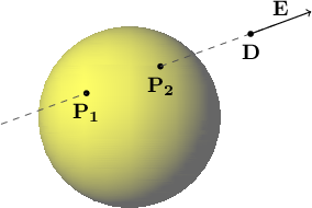
The first step, writing an equation for any point along the ray, is identical for every shape, so it is critical to understand. Fortunately, it is very simple, both conceptually and algebraically. I say the equation is parametric because it uses a parameter variable $u$ that indicates where along the ray a point is. By setting the value of $u$ to any positive number, the equation calculates the $x$, $y$, and $z$ components of a point on the ray. Let $\mathbf{D}$ be a vantage point, which is just a position vector for a fixed point in space. Let $\mathbf{E}$ be a direction vector pointing which way a ray emanates from the vantage point $\mathbf{D}$. It is important to understand that the ray extends infinitely in the direction of $\mathbf{E}$ from the vantage point $\mathbf{D}$, even though $\mathbf{E}$ is a vector with a finite magnitude.
I will write the parametric equation for a point on the ray three different ways, and explain each, just to make sure the concept is clear. The equation is most concisely expressed in vector form:
\[\mathbf{P} = \mathbf{D} + u\mathbf{E} \quad:\quad u > 0\]
where $\mathbf{P}$ is the position vector for any point along the ray. Note that $\mathbf{P}$, $\mathbf{D}$, and $\mathbf{E}$ are all vectors, but $u$ is a scalar. Also note the constraint that $u$ must be a positive real numer. If we let $u$ be zero, $\mathbf{P}$ would be at the same location as $\mathbf{D}$, the vantage point. We want to exclude the vantage point from any intersections we find, primarily to prevent us from thinking a point on a surface casts a shadow on itself. We don't allow negative values for $u$ because we would then be calculating point coordinates that are in the opposite direction as intended.
Another way to express the parametric line equation is by explicitly writing all the vector components in a single equation:
\[(P_x, P_y, P_z) = (D_x, D_y, D_z) + u(E_x, E_y, E_z)\]
Or equivalently, we can write a system of three linear scalar equations:
\[
\begin{cases}
& P_x = D_x + u E_x \\
& P_y = D_y + u E_y \\
& P_z = D_z + u E_z
\end{cases}
\]
This last form makes it especially clear how, given fixed values for the vantage point $(D_x, D_y, D_z)$ and the direction vector $(E_x, E_y, E_z)$, we can adjust $u$ to various values to select any point $(P_x, P_y, P_z)$ along the ray. Simply put, the point $\mathbf{P} = (P_x, P_y, P_z)$ is a function of the parameter $u$. Conversely, if $\mathbf{P}$ is an arbitrary point along the ray, there is a unique value of $u$ such that $\mathbf{P} = \mathbf{D} + u \mathbf{E}$. In order to find all intersections with a ray and a surface, our goal is to find all positive values of $u$ such that $\mathbf{P}$ is on that surface.
6.3 Surface equation
Now we are ready to take the second step in the solution strategy: writing a list of equations for all the surfaces on the solid object. In this example, where the solid is a sphere, there is a single equation that must be satisfied by any point on the spherical surface:
\[
(P_x - C_x)^2 + (P_y - C_y)^2 + (P_z - C_z)^2 = R^2
\]
where $\mathbf{P} = (P_x, P_y, P_z)$ is any point on the sphere (intentionally the same $\mathbf{P}$ as in the parametric ray equation above), $\mathbf{C} = (C_x, C_y, C_z)$ is the center of the sphere expressed as a position vector, and $R$ is the radius of the sphere.
6.4 Intersection of ray and surface
Step 3 in the solution strategy is to substitute the parametric ray equation into the surface equation(s). This means solving for all points $\mathbf{P}$ that are both on the ray and on one of the solid's surfaces. So we have
\[
(P_x - C_x)^2 + (P_y - C_y)^2 + (P_z - C_z)^2 = R^2
\]
with
\[
\begin{cases}
& P_x = D_x + u E_x \\
& P_y = D_y + u E_y \\
& P_z = D_z + u E_z
\end{cases}
\]
Everywhere we see $P_x$, $P_y$, or $P_z$ in the first equation, we substitute the appropriate right-hand side from the second system of linear equations. This is the key: we end up with a single equation with a single unknown, the parameter $u$.
\[
\big( (D_x + u E_x) - C_x \big)^2 +
\big( (D_y + u E_y) - C_y \big)^2 +
\big( (D_z + u E_z) - C_z \big)^2 = R^2
\]
Expanding the squared expressions, we have
\begin{align*}
& E_x^2 u^2 + 2 E_x(D_x - C_x)u + (D_x - C_x)^2 + \\
& E_y^2 u^2 + 2 E_y(D_y - C_y)u + (D_y - C_y)^2 + \\
& E_z^2 u^2 + 2 E_z(D_z - C_z)u + (D_z - C_z)^2 = R^2
\end{align*}
We can write this as a standard-form quadratic equation in $u$:
\begin{align*}
& (E_x^2 + E_y^2 + E_z^2)u^2 + \\
& 2 \big( E_x(D_x - C_x) + E_y(D_y - C_y) + E_z(D_z - C_z) \big) u + \\
& (D_x - C_x)^2 + (D_y - C_y)^2 + (D_z - C_z)^2 - R^2 \\
& = 0
\end{align*}
Like any other quadratic equation in a single unknown variable, we have a constant coefficient for the $u^2$ term, another for the $u$ term, and a constant term, all adding up to zero. If we create temporary symbols $a$, $b$, $c$ for the coefficients, letting
\[
\begin{cases}
& a = E_x^2 + E_y^2 + E_z^2 \\
& b = 2 \big( E_x(D_x - C_x) + E_y(D_y - C_y) + E_z(D_z - C_z) \big) \\
& c = (D_x - C_x)^2 + (D_y - C_y)^2 + (D_z - C_z)^2 - R^2
\end{cases}
\]
We then have the familiar quadratic equation
\[a u^2 + b u + c = 0\]
for which the solutions are
\[u = \frac{-b \pm \sqrt{b^2 - 4 a c}}{2 a}\]
Depending on the values of $a$, $b$, and $c$, the quadratic equation may have 0, 1, or 2 real solutions for $u$. These three special cases correspond to three different scenarios where a ray may miss the sphere entirely (0 solutions), may graze the sphere tangentially at one point (1 solution), or may pierce the sphere, entering at one point and exiting at another (2 solutions). The value of the expression inside the quadratic solution's square root (called the radicand) determines which of the three special cases we counter:
\[
\begin{cases}
b^2 - 4ac < 0 & \quad \textrm{0 solutions} \\
b^2 - 4ac = 0 & \quad \textrm{1 solution} \\
b^2 - 4ac > 0 & \quad \textrm{2 solutions}
\end{cases}
\]
Interestingly, and usefully for our programming, we can express the values of $a$, $b$, $c$ more concisely using vector dot products and magnitudes:
\begin{align*}
& a = \lvert \mathbf{E} \rvert ^ 2 \\
& b = 2 \mathbf{E} \cdot (\mathbf{D} - \mathbf{C}) \\
& c = \lvert \mathbf{D} - \mathbf{C} \rvert ^ 2 - R^2
\end{align*}
In the C++ code for the function Sphere::AppendAllIntersections, $\mathbf{E}$ is the function parameter direction, and $\mathbf{D}$ is the parameter vantage. The center of the sphere is inherited from the base class SolidObject; we obtain its vector value via the function call Center(). The radius of the sphere is stored in Sphere's member variable radius. So we express the calculation of the quadratic's coefficients and the resulting radicand value as:
    const Vector displacement = vantage - Center();
    const double a = direction.MagnitudeSquared();
    const double b = 2.0 * DotProduct(direction, displacement);
    const double c = displacement.MagnitudeSquared() - radius*radius;
    const double radicand = b*b - 4.0*a*c;
Once we calculate radicand, we check to see if it is less than zero. If so, we immediately know that there are no intersections with this ray and the sphere. Otherwise, we know we can take the square root of the radicand, and proceed to calculate two values for $u$. (Because it is a very rare case, we don't worry about whether the radicand is zero. Whether it is zero or positive, we calculate separate values for $u$ using the $\pm$ in the quadratic solution formula. It is faster, and harmless, to assume that there are two intersections, even if they are occasionally the same point in space.)
But it is not enough that a value of $u$ is real; we must check each $u$ value to see if it is positive. As stated before, a negative $u$ value means the intersecion point lies in the wrong direction, as shown in Figure 6.1.
|
Figure 6.1: When $u < 0$, it means the intersection is in the opposite of the intended direction $\mathbf{E}$ from the vantage point $\mathbf{D}$. In this example, there are two intersections that lie in the wrong direction from $\mathbf{D}$: At $\mathbf{P_1}$, the value of $u$ is $-2.74$, and at $\mathbf{P_2}$, $u=-1.52$. |
|
In short, if $u$ is zero, the intersection is at the vantage point, if $u$ is negative, it is behind the vantage point, and if $u$ is positive, it is in front of the vantage point. So only positive values of $u$ count as valid intersections. When $u$ is positive ($u > 0$), the larger the value of $u$, the farther away the intersection point is from the vantage point. Because of floating point rounding errors, we actually make sure that $u$ is greater than a small constant value EPSILON, not zero. This prevents erroneous intersections from being found too close to the vantage point, which would cause problems when calculating shadows and lighting. EPSILON is defined as $10^{-6}$, or one-millionth, in imager.h:
const double EPSILON = 1.0e-6;
If we find positive real solutions for $u$, we can plug each one back into the parametric ray equation to obtain the location of the intersection point:
\[\mathbf{P} = \mathbf{D} + u \mathbf{E}\]
In C++ code, this looks like:
intersection.point = vantage + u*direction;
The overloaded operators * and + for class Vector allow us to write this calculation in a natural and concise way, and because these operators are implemented as inline functions (in imager.h) they are very efficient in release/optimized builds.
6.5 Surface normal vector
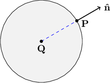
Step 4 of the solution strategy for any solid object is to calculate the surface normal unit vector at each intersection point. This unit vector will be needed for calculating the effect of any light sources shining on that point at the object's surface. In the case of a sphere, the surface normal unit vector points exactly away from the center of the sphere, as shown in Figure 6.2.
|
Figure 6.2: The surface normal vector $\mathbf{\hat{n}}$ at any point $\mathbf{P}$ on the surface of a sphere points away from the sphere's center $\mathbf{Q}$. |
|
If $\mathbf{Q}$ is the center of the sphere, $\mathbf{P}$ is the intersection point on the sphere's surface, and $\mathbf{\hat{n}}$ is the surface normal unit vector, then $\mathbf{P} - \mathbf{Q}$ is a vector that points in the same direction as $\mathbf{\hat{n}}$. We can divide the vector difference $\mathbf{P} - \mathbf{Q}$ by its magnitude $\lvert \mathbf{P} - \mathbf{Q} \rvert$ to convert it to the unit vector $\mathbf{\hat{n}}$:
\[
\mathbf{\hat{n}} = \frac{\mathbf{P} - \mathbf{Q}}{\lvert \mathbf{P} - \mathbf{Q} \rvert}
\]
In C++ code, we can use the method UnitVector in class Vector to do the same thing:
    intersection.surfaceNormal =
        (intersection.point - Center()).UnitVector();
6.6 Filling in the Intersection struct
Step 5 has been mostly accomplished already — we have calculated the intersection point and the surface normal unit vector, and both are stored in the struct Intersection variable called intersection. But we also need to store the square of the distance between the intersection point and the vantage point inside intersection. The distance squared calculation and the intersection point calculation both involve the term $u\mathbf{E}$ (or u * direction in C++), so it is a bit more efficient to calculate the product once and store it in a temporary variable of type Vector. After filling out all the fields of the local variable intersection, we must remember to insert it into the output list parameter intersectionList:
intersectionList.push_back(intersection);
6.7 C++ sphere implementation
The entire function Sphere::AppendAllIntersections is shown here, just as it appears in sphere.cpp:
void Sphere::AppendAllIntersections(
    const Vector& vantage,
    const Vector& direction,
    IntersectionList& intersectionList) const
{
    // Calculate the coefficients of the quadratic equation
    //     au^2 + bu + c = 0.
    // Solving this equation gives us the value of u
    // for any intersection points.
    const Vector displacement = vantage - Center();
    const double a = direction.MagnitudeSquared();
    const double b = 2.0 * DotProduct(direction, displacement);
    const double c = displacement.MagnitudeSquared() - radius*radius;

    // Calculate the radicand of the quadratic equation solution formula.
    // The radicand must be non-negative for there to be real solutions.
    const double radicand = b*b - 4.0*a*c;
    if (radicand >= 0.0)
    {
        // There are two intersection solutions, one involving
        // +sqrt(radicand), the other -sqrt(radicand).
        // Check both because there are weird special cases,
        // like the camera being inside the sphere,
        // or the sphere being behind the camera (invisible).
        const double root = sqrt(radicand);
        const double denom = 2.0 * a;
        const double u[2] = {
            (-b + root) / denom,
            (-b - root) / denom
        };

        for (int i=0; i < 2; ++i)
        {
            if (u[i] > EPSILON)
            {
                Intersection intersection;
                const Vector vantageToSurface = u[i] * direction;
                intersection.point = vantage + vantageToSurface;

                // The normal vector to the surface of
                // a sphere is outward from the center.
                intersection.surfaceNormal =
                    (intersection.point - Center()).UnitVector();

                intersection.distanceSquared =
                    vantageToSurface.MagnitudeSquared();

                intersection.solid = this;
                intersectionList.push_back(intersection);
            }
        }
    }
}
6.8 Switching gears for a while
We will look at the algebraic solutions for other shapes in later chapters, but first we need to take a look at how these lists of intersection objects are used to help implement an optical simulator. We have already discussed how the ray tracing algorithm looks for intersections between camera rays and solid objects. In the next chapter we begin exploring how the ray tracing algorithm assigns a color to an intersection it finds, based on optical processes like reflection and refraction.
Copyright © 2013 by
Don Cross.
All Rights Reserved.