Chapter 5: C++ Code for Ray Tracing
5.1 Platforms and redistribution
This book is accompanied by C++ code that you can download for free and build as-is or modify. The code will build and run without modification on Windows, Linux, and Mac OS X. I built it on Windows 7 using Microsoft Visual Studio 2008, and on both Ubuntu Linux 9.10 and Mac OS X 10.8.2 using a simple script that launches g++, the C++ front end for the GNU compiler suite (or LLVM on OS X). All of my code is open source. You may use and re-distribute this code (or portions of it) for your own private, educational, or commercial purposes, so long as the comment blocks at the front of each source file with my name, web site address, and copyright and legal notices are left intact. See the legal notices at the front of any of the source files (.cpp or .h) for more details.
Please note that I am not the author of the files lodepng.h and lodepng.cpp for writing PNG formatted image files; these were created by Lode Vandevenne. For more information about LodePNG, please visit http://lodev.org/lodepng. Both LodePNG and my ray tracing code are provided with similar open source licenses.
5.2 Downloading and installing
Download the zip file
http://cosinekitty.com/raytrace/rtsource.zip
to a convenient location on your hard drive. The easiest way is to use your web browser and let it prompt you for the location where you want to save the zip file. Alternatively, in Linux or OS X you can go into a terminal window (where you will need to end up soon anyway) and enter the following command from somewhere under your home folder:
curl http://cosinekitty.com/raytrace/rtsource.zip -o rtsource.zip
After downloading the file, unzip its contents. If there is an option in your unzip program to preserve the subdirectory structure encoded in the zip file, be sure to enable it. Linux or OS X users can use the unzip command:
unzip rtsource.zip
This will create a new subdirectory called raytrace beneath your current directory that contains everything you need to follow along with the rest of this book.
5.3 Building on Windows
Use Microsoft Visual C++ to open the solution file
...\raytrace\raytrace.sln
where ... represents the path where you unzipped rtsource.zip. Then choose the menu item Build, followed by Batch Build to compile all the code. Check the boxes for both Debug and Release configurations, then click the Build button. The code should compile and link with no warnings and no errors.
5.4 Getting ready to build under OS X
If you do any software development for the Macintosh, you have probably already installed some version of Apple's integrated development environment, Xcode. However, your machine may or may not be ready to build C++ programs from the command line. To find out, open a Terminal window and type the command g++. If you get a "command not found" error, you will need to follow a couple of steps to get the command-line build tools installed. Here is what I did using Xcode 4.6:
- Open up Xcode.
- Under the Xcode menu at the top of your screen, choose Preferences.
- A box will appear. Choose the Downloads tab.
- Look for a "Command Line Tools" entry. Click the Install button to the right of it.
- Wait for the command line tools to download and install.
- Go back into your Terminal window. When you enter the g++ command again, it should no longer say "command not found" but should instead say something like i686-apple-darwin11-llvm-g++-4.2: no input files.
If you do not have Xcode installed, and you don't want to download 1.65 GB just to build from the command line, here is a more palatable alternative. You will need an Apple ID, but you can create one for free. Once you have an Apple ID, take a look at the Downloads for Apple Developers page whose URL is listed below and find the Command Line Tools package appropriate for your version of OS X. The download will be much smaller (about 115 MB or so) and will cost you nothing.
https://developer.apple.com/downloads/index.action
Once you get g++ installed, you are ready to proceed to the next section.
5.5 Building on Linux and OS X
Go into a command prompt (terminal window) and change to the directory where you unzipped rtsource.zip. Then you will need to go into the two levels deep of directories both named raytrace:
cd raytrace/raytrace
The first time before you build the code for Linux, you will need to grant permission to run the build script as an executable:
chmod +x build
And finally, build the code:
./build
You should see the computer appear to do nothing for a few seconds, then return to the command prompt. A successful build will not print any warnings or errors, and will result in the executable file raytrace in the current directory: if you enter the command
ls -l raytrace
you should see something like
-rwxr-xr-x 1 dcross dcross 250318 2012-10-29 15:17 raytrace
5.6 Running the unit tests
Once you get the C++ code built on Windows, Linux, or OS X, running it is very similar on any of these operating system. On Windows the executable will be
raytrace\Release\raytrace.exe
On Linux or OS X, it will be
raytrace/raytrace/raytrace
In either case, you should run unit tests to generate some sample PNG images to validate the built code and see what kinds of images it is capable of creating. The images generated by the unit tests will also be an important reference source for many parts of this book.
Go into a command prompt (terminal window) and change to the appropriate directory for your platform's executable, as explained above. Then run the program with the test option. (You can always run the raytrace program with no command line options to display help text that explains what options are available.) On Linux or OS X you would enter
./raytrace test
And on Windows, you would enter
raytrace test
You will see a series of messages that look like this:
Wrote donutbite.png
When finished, the program will return you to the command prompt. Then use your web browser or image viewer software to take a peek at the generated PNG files. On my Windows 7 laptop, here is the URL I entered in my web browser to see all the output files.
file:///C:/don/dev/trunk/math/block/raytrace/raytrace/
On my OS X machine, the URL looks like this:
file:///Users/don/raytrace/raytrace/
Yours will not be exactly the same as these, but hopefully this gets the idea across.
If everything went well, you are now looking at a variety of image files that have .png extensions. These image files demonstrate many of the capabilities of the raytrace program. Take a few moments to look through all these images to get a preview of the mathematical and programming topics to come.
5.7 Example of creating a ray-traced image
Let's dive into the code and look at how the double-torus image in Figure 1.1 was created. Open up the source file main.cpp with your favorite text editor, or use Visual Studio's built-in programming editor. In Visual Studio, you can just double-click on main.cpp in the Solution Explorer; main.cpp is listed under Source Files. Using any other editor, you will find main.cpp in the directory raytrace/raytrace. Once you have opened main.cpp, search for the function TorusTest. It looks like this:
void TorusTest(const char* filename, double glossFactor)
{
    using namespace Imager;

    Scene scene(Color(0.0, 0.0, 0.0));

    const Color white(1.0, 1.0, 1.0);
    Torus* torus1 = new Torus(3.0, 1.0);
    torus1->SetMatteGlossBalance(glossFactor, white, white);
    torus1->Move(+1.5, 0.0, 0.0);

    Torus* torus2 = new Torus(3.0, 1.0);
    torus2->SetMatteGlossBalance(glossFactor, white, white);
    torus2->Move(-1.5, 0.0, 0.0);
    torus2->RotateX(-90.0);

    SetUnion *doubleTorus = new SetUnion(
        Vector(0.0, 0.0, 0.0),
        torus1,
        torus2
    );

    scene.AddSolidObject(doubleTorus);

    doubleTorus->Move(0.0, 0.0, -50.0);
    doubleTorus->RotateX(-45.0);
    doubleTorus->RotateY(-30.0);

    // Add a light source to illuminate the objects
    // in the scene; otherwise we won't see anything!
    scene.AddLightSource(
        LightSource(
            Vector(-45.0, +10.0, +50.0),
            Color(1.0, 1.0, 0.3, 1.0)
        )
    );

    scene.AddLightSource(
        LightSource(
            Vector(+5.0, +90.0, -40.0),
            Color(0.5, 0.5, 1.5, 0.5)
        )
    );

    // Generate a PNG file that displays the scene...
    scene.SaveImage(filename, 420, 300, 5.5, 2);
    std::cout << "Wrote " << filename << std::endl;
}
Don't worry too much about any details you don't understand yet — everything will be explained in great detail later in this book. For now, just notice these key features:
- We create a local variable of type Scene. We specify that its background color is Color(0.0, 0.0, 0.0), which is black.
- We create a Torus object called torus1 and move it to the right (in the $+x$ direction) by 1.5 units.
- We create another Torus called torus2, move it left by 1.5 units, and rotate it $90°$ clockwise around its $x$-axis (technically, about an axis parallel to the $x$-axis that passes through the object's center, but more about that later). Rotations using negative angle values, as in this case, are clockwise as seen from the positive axis direction; positive angle values indicate counterclockwise rotations.
- We create a SetUnion of torus1 and torus2. For now, just think of SetUnion as a container that allows us to treat multiple visible objects as a single entity. This variable is called doubleTorus.
- We call scene.AddSolidObject() to add doubleTorus to the scene. The scene is responsible for deleting the object pointed to by doubleTorus when scene gets destructed. The destructor Scene::\textasciitilde Scene() will do this automatically when the code returns from the function TorusTest. That destructor is located in imager.h.
- The doubleTorus is moved 50 units in the $-z$ direction, away from the camera and into its prime viewing area. (More about the camera later.) Then we rotate doubleTorus, first $45°$ around its center's $x$-axis, then $30°$ around its center's $y$-axis. Both rotations are negative (clockwise). Note that we can move and rotate objects either before or after adding them to the Scene; order does not matter.
- We add two point light sources to shine on the double torus, one bright yellow and located at $(-45, 10, 50)$, the other a dimmer blue located at $(5, 90, -40)$. As noted in the source code's comments, if we forget to add at least one light source, nothing but a solid black image will be generated (not very interesting).
- Finally, now that the scene is completely ready, with all visible objects and light sources positioned as intended, we call scene.SaveImage() to ray-trace an image and save it to a PNG file called torus.png. This is where almost all of the run time is: doing all the ray tracing math.
5.8 The Vector class
The Vector class represents a vector in three-dimensional space. We use double-precision floating point for most of the math calculations in the ray tracing code, and the members x, y, and z of class Vector are important examples of this. In addition to the raw component values stored as member variables, class Vector has two constructors, some member functions, and some helper inline functions (including overloaded operators). The default constructor initializes a Vector to $(0, 0, 0)$. The other constructor initializes a Vector to whatever $x$, $y$, $z$ values are passed into it.
The member function MagnitudeSquared returns the square of a vector's length, or $x^2 + y^2 + z^2$, and Magnitude returns the length itself, or $\sqrt{x^2 + y^2 + z^2}$. MagnitudeSquared is faster when code just needs to compare two vectors to see which is longer/shorter, because it avoids the square root operation as needed in Magnitude.
The UnitVector member function returns a vector that points in the same direction as the vector it is called on, but whose length is one. UnitVector does not modify the value of the original Vector object that it was called on; it returns a brand new, independent instance of Vector that represents a unit vector.
Just after the declaration of class Vector are a few inline functions and overloaded operators that greatly simplify a lot of the vector calculation code in the ray tracer. We can add two vector variables by putting a "+" between them, just like we could with numeric variables:
    Vector a(1.0, 5.0, -3.2);
    Vector b(2.0, 3.0, 1.0);
    Vector c = a + b;    // c = (3.0, 8.0, -2.2)
Likewise, the "-" operator is overloaded for subtraction, and "*" allows us to multiply a scalar and a vector. The inline function DotProduct accepts two vectors as parameters and returns the scalar dot product of those vectors. CrossProduct returns the vector-valued cross product of two vectors.
5.9 struct LightSource
This simple data type represents a point light source. It emits light of a certain color (specified by red, green, and blue values) in all directions from a given point (specified by a position vector). At least one light source must be added to a Scene, or nothing but a black silhouette will be visible against the Scene's background color. (If that background color is also black, the rendered image will be completely black.) Often, a more pleasing image results from using multiple light sources with different colors positioned so that they illuminate objects from different angles. It is also possible to position many LightSource instances near each other to produce an approximation of blurred shadows, to counteract the very sharp shadows created by a single LightSource.
5.10 The SolidObject class
The abstract class SolidObject is the base class for all the three-dimensional bodies that this ray-tracing code draws. It defines methods for rotating and moving solid objects to any desired orientation and position in a three-dimensional space. It also specifies a contract by which calling code can determine the shape of its exterior surfaces, a method for determining whether a body contains a given point in space, and methods for determining the optical properties of the body.
All SolidObject instances have a center point, about which the object rotates via calls to RotateX, RotateY, and RotateZ. These methods rotate the entire object about the center point by the specified number of degrees counterclockwise as seen looking at that center point from the positive direction along the specified axis. For example, RotateX(15.0) will rotate the object $15°$ counterclockwise around a line parallel to the $x$-axis that passes through the object's center point, as seen from the $+x$ direction. To rotate $15°$ clockwise instead, you can do Rotate(-15.0).
The Translate method moves the object by the specified $\Delta x$, $\Delta y$, and $\Delta z$ amounts. The Move methods are similar, but they move an object such that its center point lands at the specified location. In other words, the parameters to Translate are changes in position, but the parameters to Move are absolute coordinates.
5.11 SolidObject::AppendAllIntersections
This member function is of key importance to the ray tracing algorithm. It is a pure virtual method, meaning it must be implemented differently by any derived class that creates a visible shape in a rendered image. The caller of AppendAllIntersections passes in two vectors that define a ray: a vantage point (a position vector that specifies a location in space from which the ray is drawn) and a direction vector that indicates which way the ray is aimed. AppendAllIntersections generates zero or more Intersection structs, each of which describes the locations (if any) where the ray intersects with the opaque exterior surfaces of the solid object. The new intersections are appended to the list parameter intersectionList, which may already contain other intersections before AppendAllIntersections is called.
As an example, the class Sphere, which derives from SolidObject, contains a method Sphere::AppendAllIntersections that may determine that a particular direction from a given vantage point passes through the front of the Sphere at one point and emerges from the back of the Sphere at another point. In this case, it inserts two extra Intersection structs at the back of intersectionList.
5.12 struct Intersection
The Intersection struct is a "plain old data" (POD) type for runtime efficiency. This means that any code that creates an Intersection object must take care to initialize all its members. Any members left uninitialized will have invalid default values. Here are the members of Intersection:
- distanceSquared : The square of the distance from the vantage point to the intersection point, as traveled along the given direction. As mentioned earlier, squared distances work just fine for comparing two or more distances against each other, without the need for calculating a square root.
- point : The position vector that represents the point in space where an intersection with the surface of an object was found.
- surfaceNormal : A unit vector (again, a vector whose length is one unit) that points outward from the interior of the object, and in the direction perpendicular to the object's surface at the intersection point.
- solid : A pointer to the solid object that the ray intersected with. Depending on situations which are not known ahead of time, this object may or may not need to be interrogated later for more details about its optical properties at the intersection point or some other point near the intersection.
- context : Most of the time, this field is not used, but some classes (e.g., class TriangleMesh, which is discussed later) need a way to hold extra information about the intersection point to help them figure out more about the optical properties there later. For the majority of cases where context is not needed, it is left as a null pointer.
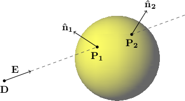
Figure 5.1 shows a vantage point $\mathbf{D}$ and a direction vector $\mathbf{E}$ which points along an infinite ray that intersects a sphere in two places, $\mathbf{P_1}$ and $\mathbf{P_2}$. The surface normal unit vectors $\mathbf{\hat{n}_1}$ and $\mathbf{\hat{n}_2}$ each point outward from the sphere and in a direction perpendicular to the sphere's surface at the respective intersection points $\mathbf{P_1}$ and $\mathbf{P_2}$.
|
Figure 5.1: A direction vector $\mathbf{E}$ from a vantage point $\mathbf{D}$ tracing along an infinite ray. The ray intersects the sphere in two places, $\mathbf{P_1}$ and $\mathbf{P_2}$, with $\mathbf{\hat{n}_1}$ and $\mathbf{\hat{n}_2}$ as their respective surface normal unit vectors. |
|
5.13 Scene::SaveImage
We encountered this method earlier when we looked at the function TorusTest in main.cpp. Now we are ready to explore in detail how it works. Scene::SaveImage is passed an output PNG filename and integer width and height values that specify the dimensions of a rectangular image to create, both expressed in pixels. The method simulates a camera point located at the origin — the point $(0, 0, 0)$ — and maps every pixel to a point on an imaginary screen that is offset from that camera point. The camera is aimed in the $-z$ direction (not the $+z$ direction) with the $+x$ axis pointing to the right and the $+y$ axis pointing upward. This way of aiming the camera allows the three axes to obey the right-hand rule while preserving the familiar orientation of $+x$ going to the right and $+y$ going up. Any visible surfaces in a scene therefore must have negative $z$ values.
Our simulated camera works just like a pinhole camera, only we want it to create a right-side-up image, not an image that is backwards and upside-down. One way to accomplish this is to imagine that the pinhole camera's screen is translucent (perhaps made of wax paper) and that we are looking at it from behind while hanging upside-down.
There is an equivalent way to conceive of this apparatus so as to obtain the same image, without the awkwardness of hanging upside-down: instead of a translucent screen behind the camera point, imagine a completely invisible screen in front of the camera point. We can still break this screen up into pixels, only this time we imagine rays that start at the camera point and pass through each pixel on the screen. Each ray continues through the invisible screen and out into the space beyond, where it may or may not strike the surface of some object. Because all objects in this ray tracer are completely opaque, whichever point of intersection (if any) is closest to the camera will determine the color of the screen pixel that the ray passed through.
It doesn't matter which of these two models you imagine; the formulas for breaking up the screen into pixels will be the same either way, and so will the resulting C++ code. If you open up the source file scene.cpp and find the code for Scene::SaveImage, you will see that it requires two other arguments in addition to the filename, pixel width, and pixel height: one called zoom and the other called antiAliasFactor. The zoom parameter is a positive number that works like the zoom lens on a camera. If zoom has a larger numeric value, SaveImage will create an image that includes a wider and taller expanse of the scenery — the objects will look smaller but more will fit inside the screen. Passing a smaller value for zoom will cause objects to appear larger by including a smaller portion of the scene.
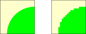
The final parameter, antiAliasFactor, is an integer that allows the caller to adjust the compromise between faster rendering speed and image quality. We need to pause here to consider a limitation of ray tracing. Because there are only a finite number of pixels in any digital image, and ray-traced images follow the path of a single ray for each pixel on the screen, it is possible to end up with unpleasant distortion in the image known as aliasing. Figure 5.2 shows an example of aliasing. On the left is an image of a quarter-circle. On the right is how the image would appear when rendered using a grid of 20 pixels wide by 20 pixels high.
|
Figure 5.2: An idealized image on the left, and aliasing of it on the right when converted to a $20\times20$ grid of pixels. |
|
The jagged boundary, sometimes likened to stair steps, is what we mean by the word aliasing. It results from the all-or-nothing approach of forcing each pixel to take on the color of a single object. The antiAliasFactor provides a way to reduce (but not eliminate) aliasing by passing multiple rays at slightly different angles through each pixel and averaging the color obtained for these rays into a single color that is assigned to the pixel.
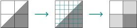
For example, passing antiAliasingFactor = 3 will break each pixel into a $3 \times 3$ grid, or 9 rays per pixel, as shown in Figure 5.3.
|
Figure 5.3: Anti-aliasing of a $2 \times 2$ image by breaking each pixel into a $3 \times 3$ grid and averaging the colors. |
|
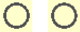
Figure 5.4 shows a comparison of the same scene imaged with antiAliasFactor set to 1 (i.e., no anti-aliasing) on the left, and 5 on the right.
|
Figure 5.4: A scene without anti-aliasing (left) and with anti-aliasing (right). |
|
There is a price to pay for using anti-aliasing: it makes the images take much longer to generate. In fact, the execution time increases as the square of the antiAliasFactor. You will find that setting antiAliasFactor to 3 will cause the image rendering to take 9 times as long, setting it to 4 will take 16 times as long, etc. There is also diminishing return in image quality for values much larger than 4 or 5. When starting the code to create a new image, I recommend starting with antiAliasFactor = 1 (no anti-aliasing) until you get the image framing and composition just the way you like. Then you can increase antiAliasFactor to 3 or 4 for a prettier final image. This will save you some time along the way.
5.14 Scene::TraceRay
In Scene::SaveImage you will find the following code as the innermost logic for determining the color of a pixel:
    // Trace a ray from the camera toward the given direction
    // to figure out what color to assign to this pixel.
    pixel.color = TraceRay(
        camera,
        direction,
        ambientRefraction,
        fullIntensity,
        0);
TraceRay embodies the very core of this ray tracer's optical calculation engine. Four chapters will be devoted to how it simulates the physical behavior of light interacting with matter, covering the mathematical details of reflection and refraction. For now, all you need to know is that this function returns a color value that should be assigned to the given pixel based on light coming from that point on an object's surface.
5.15 Saving the final image to disk
After adding up the contributions of reflection from a point and refraction through that point, the function Scene::TraceRay returns the value of colorSum to the caller, Scene::SaveImage. This color value is used as the color of the pixel associated with the camera ray that intersected with the given point. SaveImage continues tracing rays from the camera to figure out the color of such pixels that have a surface intersection point along their line of sight. When SaveImage has explored every pixel in the image and has determined what colors they all should have, it performs three post-processing steps before saving an image to disk:
- Sometimes tracing the ray through a pixel will lead to an ambiguity where multiple intersections are tied for being closest to a vantage point. The vantage point causing the problem may be the camera itself, or it might be a point on some object that the light ray reflects from or refracts through. To avoid complications that will be explained later, such pixels are marked and skipped in the ray tracing phase. In post-processing, SaveImage uses surrounding pixel colors to approximate what the ambiguous pixel's color should be.
- If antiAliasFactor is greater than one, SaveImage averages square blocks of pixels into a single pixel value, as discussed in the earlier section on anti-aliasing. This reduces both the pixel width and the pixel height by the antiAliasFactor.
- The floating point color values of each pixel, having an unpredictable range of values, must be converted to integers in the range 0 to 255 in order to be saved in PNG format. SaveImage searches the entire image for the maximum value of any red, green, or blue color component. That maximum floating point value (let's call it M) is used to linearly scale the color components of every pixel to fit in the range 0 to 255:
    R = round(255 * r / M)
    G = round(255 * g / M)
    B = round(255 * b / M)
where r, g, b are floating point color components, and R, G, B are integer values in the range of a byte, or 0 to 255.
Unlike the pseudocode above, the C++ code performs the second calculation using a function called ConvertPixelValue, which has logic that ensures the result is always clamped to the inclusive range 0 to 255:
    // Convert to integer red, green, blue, alpha values,
    // all of which must be in the range 0..255.
    rgbaBuffer[rgbaIndex++] = ConvertPixelValue(sum.red,   maxColorValue);
    rgbaBuffer[rgbaIndex++] = ConvertPixelValue(sum.green, maxColorValue);
    rgbaBuffer[rgbaIndex++] = ConvertPixelValue(sum.blue,  maxColorValue);
    rgbaBuffer[rgbaIndex++] = OPAQUE_ALPHA_VALUE;
As a quirk in the rgbaBuffer, each pixel requires a fourth value called alpha, which determines how transparent or opaque the pixel is. PNG files may be placed on top of some background image such that they mask some parts of the background but allow other parts to show through. This ray tracing code makes all pixels completely opaque by setting all alpha values to OPAQUE_ALPHA_VALUE (or 255).
After filling in rgbaBuffer with single-byte values for red, green, blue, and alpha for each pixel in the image (a total of 4 bytes per pixel), SaveImage calls Lode Vandevenne's LodePNG code to write the buffer to a PNG file:
    // Write the PNG file
    const unsigned error = lodepng::encode(
        outPngFileName,
        rgbaBuffer,
        pixelsWide,
        pixelsHigh);
You now have a general idea of how a scene is broken up into pixels and converted into an image that can be saved as a PNG file. The code traces rays of light from the camera point toward thousands of vector directions, each time calling TraceRay. That function figures out what color to assign to the pixel associated with that direction from the camera point. In upcoming chapters we will explore TraceRay in detail to understand how it computes the intricate behavior of light as it interacts with physical matter. But first we will study an example of solving the mathematical problem of finding an intersection of a ray with a simple shape, the sphere.
Copyright © 2013 by
Don Cross.
All Rights Reserved.